Outputs

Outputs from Parthenon are controlled via <parthenon/output*> blocks, where * should be replaced by a unique integer for each block.

Various output types are supported for writing both raw data (e.g., in openPMD/ADIOS2/BP5 or HDF5 format) andprocessed data (like high level aggregated history files or histograms), see following subsections for more details. While HDF5 has been the default in the past, openPMD/ADIOS2/BP5 is expected to become the default in the near term future given its features, flexiblity, and significantly improved perforance (especially at scale). Advanced features like slices or coarse graining are only supported in openPMD outputs.

The frequency of outputs can be controlled for each block separately and can be triggered by either (simulation) time or cycle, i.e.,

• dt = 0.1 means that the output for the block is written every 0.1 in simulation time.

• dn = 100 means that the output for the block is written every 100 cycles.

Note that only one option can be chosen for a given block. To disable an output block without removing it from the input file set the block’s dt < 0.0 and dn < 0 (which is also happening by default if the paramter is not provided in the input file).

In addition to time or cycle based outputs, two additional options to trigger outputs (applies to OpenPMD, HDF5, restart, and histogram outputs) exist.

• Signaling: If Parthenon catches a signal, e.g., SIGALRM which is often sent by schedulers such as Slurm to signal a job of exceeding the job’s allocated walltime, Parthenon will gracefully terminate and write output files with a final id rather than a number. This also applies to the Parthenon internal walltime limit, e.g., when executing an application with the -t HH:MM:SS parameter on the command line.

• File trigger: If a user places a file with the name output_now in the working directory of a running application, Parthenon will write output files with a now id rather than a number. After the output is being written the output_now file is removed and the simulation continues normally. The user can repeat the process any time by creating a new output_now file.

Note, in both cases the original numbering of the output will be unaffected and the final and now files will be overwritten each time without warning.

openPMD

Parthenon supports writing outputs in the “Open Standard for Particle-Mesh Data”, openPMD. While openPMD supports various backends only the ADIOS2 IO framework is currently supported/tested with files being writen in BP5 format.

The most simple output block for openPMD output is

<parthenon/output6>
file_type  = openpmd    # write data in openPMD format
dt         = 0.125      # time increment between outputs

and will produce outputs in directories named parthenon.out6.#####.bp where the 6 (in the output block header is arbitrary and used as default value in the resulting directory name) and ##### an increasing zero-padded integer that is increased for each output written.

Restarting from outputs using these minimal, simple block is supported by default (i.e., it contains all the information for restarting a simulation, such as independent field, mesh structure, input file, and other parameters).

More complex configurations are possible, e.g.,

<parthenon/output5>
file_type  = openpmd           # write data in openPMD format
dt         = 0.125             # time increment between outputs
id         = compressed        # arb. string used in resulting directory name
backend_config  = openpmd.toml # path to external config file controlling IO behavior

Here, the resulting outputs will be written to parthenon.compressed.#####.bp directories and an external config file (arbitrarily named openpmd.toml) is parsed to tune IO behavior (like performance or compression). This might be particuarly relevant at scale or for reduced outputs. For example, it could be useful to tune the total number of files being written to to the number of storage servers/blocks for large outputs or reduce the number of files to just one for simple, reduced outputs (like slices where some ranks may not write any data at all). By default ADIOS2 uses the “TwoLevelShm” aggegration approach where only one rank per compute node write data (to a unique file for each rank in the output folder), see the ADIOS2 doc. To control this (even at runtime) and enable compression for outputs, a potential openpmd.toml file could look like

[adios2.engine.parameters]
NumSubFiles = "1"

# use double brackets to indicate lists
[[adios2.dataset.operators]]
type = "blosc"

# specify parameters for the current operator
[adios2.dataset.operators.parameters]
clevel = "1"
doshuffle = "BLOSC_BITSHUFFLE"

and results in data being written to a single file (per output) and compressed using the BLOSC algorithm. Various compression algorithms (including very efficient, but lossy ones) are supported. Given that they are handled by ADIOS2 (and libraries compiled into ADIOS2) and are thus external to Parthenon, the documenations of those libraries applies.

Warning

While openPMD supports writing attributes only from a subset of ranks, do not use this option for Parthenon outputs as some attributes/metadata may only be written from a subset of ranks and, therefore, missing if those ranks are not included in the actual writing process. The architecture of ADIOS2 already allows to performantly write attributes at scale (contrary to a potential bottleneck in HDF5 outputs).

Slices and coarsened outputs

openPMD outputs in Parthenon support reduced data outputs in form of slices (i.e., 2D cuts in a 3D domain at a given coodinate value) and coarsened (i.e., only writing a subset of cells). Note that coarsening only supports factors in powers of two (i.e., picking n-th cell in each direction) and no interpolation is done. In addition, data can be written in single precision. All three options are mix and match and support multilevel meshes. These kind of outputs can dramatically reduce output volume (often without sacrificing fidelity for post processing), for example, a 3D simulation coarse grained by a factor of 2 and written in single precision uses only 1/16th disk storage (compared to the corresponding restart output). Thus, they especially suitable for analysis pipelines that benefit from high temporal resolution or animations/movies.

An output block for the latter example may look like

<parthenon/output4>
file_type         = openpmd
dt                = 0.05
id                = single_coarse # arb. id for easy identification
single_precision_output = true    # write data using float32
# dump every n-th cell (in each dim), only powers of two are supported
coarsening_factor = 2

An output block for slices may look like

<parthenon/output10>
file_type         = openpmd
dt                = 0.05        # frequency of outputs
id                = sl.x1.0.5   # arb. id for easy identification
output_type       = x1slice     # fixed axis of slice. Options: x1slice, x2slice, x3slice
slice_loc         = 0.5         # location of the slice
backend_config    = single_file.toml  # (optional) runtime IO config

where the backend configuration is optional (but recommended at scale to prevent a large number of empty files being created from nodes that do not handle blocks intersecting with the slice) ensuring that only a single file is written (single_file.toml):

[adios2.engine.parameters]
NumSubFiles = "1"

HDF5

Parthenon allows users to select which fields are captured in the HDF5 (.phdf) dumps at runtime. In the input file, include a <parthenon/output*> block, list of variables, and specify file_type = hdf5. A dt parameter controls the frequency of outputs for simulations involving evolution. If the optional parameter single_precision_output is set to true, all variable data will be written in single precision. A <parthenon/output*> block might look like

<parthenon/output1>
file_type = hdf5
write_xdmf = true # Determines whether xdmf annotations are output
# nonexistent variables/swarms are ignored
variables = density, velocity, & # comments are still ok
            energy               # notice the & continuation character
                                 # for multiline lists
swarms = tracers, photons  # Particle swarms
swarm_variables = x, y, z  # swarm variables output for every swarm

# Each swarm can sepcify in a separate list which additional
# variables it would like to output.
tracers_variables = x, y, z, rho, id
photons_variables = x, y, z, frequency

dt = 1.0
file_number_width = 6 # default: 5
use_final_label = true # default: true

# Sparse variables may not be allocated on every block. By default
# parthenon outputs de-allocated variables as 0 in the output
# file. However, it is often convenient to output them as NaN
# instead, marking deallocated and allocated but zero as
# separate. This flag turns this functionality on.
sparse_seed_nans = false # default false

# Optionally, you may specify a MeshData name to output from.
# This is unique per output block. The default is "base"
# which is usually what you want.
# Note that SWARMS only exist in the base MeshData register
# and so this has no effect on swarm data.
meshdata_name = base

# You can choose to optionally output ghost zones if you'd like to
# inspect them. Default is false.
ghost_zones = false

This will produce an hdf5 (.phdf) output file every 1 units of simulation time containing the density, velocity, and energy of each cell. The files will be identified by a 6-digit ID, and the output file generated upon completion of the simulation will be labeled *.final.* rather than with the integer ID.

HDF5 and restart files write variable field data with inline compression by default. This is especially helpful when there are sparse variables allocated only in a few blocks, because all other blocks would write zeros of these variables, which can drastically increase output file size (and decrease I/O performance) without compression. The optional parameter hdf5_compression_level can be used to set the compression level (between 1 and 9, default is 5). If parthenon is compiled with support for compression, this also enables (logical) chunking of the data in blocks of nx1*nx2*nx3. Compression (and thus chunking) can be disabled altogether with the CMake build option PARTHENON_DISABLE_HDF5_COMPRESSION. See the Building Parthenon for more details.

Tuning HDF5 Performance

Tuning IO parameters can be passed to Parthenon through the use of environment variables. Available environment variables are:

Environment Variable	Initial State	Value Type	Description
H5_sieve_buf_size H5_meta_block_size H5_alignment_threshold H5_alignment_alignment H5_defer_metadata_flush MPI_access_style MPI_collective_buffering MPI_cb_block_size MPI_cb_buffer_size	disabled disabled disabled disabled disabled enabled disabled N/A N/A	int int int int int string int int int	Sets the maximum size of the data sieve buffer, in bytes. The value should be equal to a multiple of the disk block size. If no value is set then the default is 256 KiB. Sets the minimum metadata block size, in bytes. If no value is set then the default is 8 MiB. May help performance if enabled. The threshold value, in bytes, of H5Pset_alignment. Setting to 0 forces everything to be aligned. If a value is not set then the default is 0. Setting the environment variable automatically enables alignment. The alignment value, in bytes, of H5Pset_alignment. If a value is not set then the default is 8 MiB. Setting the environment variable automatically enables alignment. H5Pset_alignment sets the alignment properties of a file access property list. Choose an alignment that is a multiple of the disk block size, enabling this usually shows better performance on parallel file systems. However, enabling may increase the file size significantly. Value of 1 enables deferring metadata flush. Value of 0 disables. Experiment with before using. Specifies the manner in which the file will be accessed until the file is closed. Default is “write_once” Value of 1 enables MPI collective buffering. Value of 0 disables. Experiment with before using. Sets the block size, in bytes, to be used for collective buffering file access. Default is 1 MiB. Sets the total buffer space, in bytes, that can be used for collective buffering on each target node, usually a multiple of cb_block_size. Default is 4 MiB.

Corehdf5

Sometimes, usually for debugging purposes, you may wish to dump every variable that parthenon is aware of. To do so, request a corehdf5 file. These files are identical to hdf5 output files, but parthenon automatically selects every variable and swarm variable it is aware of for output. A relevant output block might look like:

<parthenon/output3>
file_type = corehdf5
dt = 1.0
write_xdmf = false

this will produce an hdf5 (.chdf) output file every 1 unit of simulation time that can be read with standard visualization tools but contains everything.

Warning

It is unwise to output corehdf5 files routinely as they might be very large. These should be used only strategically.

Restart Files (openPMD and HDf5)

Parthenon allows users to output restart files for restarting a simulation. The restart file captures the input file, so no input file is required to be specified. Parameters for the input can be overridden in the usual way from the command line. At a future date we will allow for users the ability to extensively edit the parameters stored within the restart file. Restart files can either be written in openPMD format or in HDF5 format.

In the input file, include a <parthenon/output*> block and specify file_type = rst (for HDF5) or file_type = openpmd (for openPMD). A dt parameter controls the frequency of outputs for simulations involving evolution. A <parthenon/output*> block might look like

<parthenon/output7>
file_type = rst
dt = 1.0

This will produce an HDF5 (.rhdf) output file every 1 units of simulation time that can be used for restarting the simulation. Note, that the key difference between the “standard” HDF5 output files (with .phdf suffix) and restart HDF5 files are enforced settings for the latter, such as writing all independent variables and writing data in the native simulation precision. For openPMD output files there is no distinction in naming.

To use this restart file, simply specify the restart file with a -r /PATH/TO/RESTART_OUTPUT at the command line. If both -r /PATH/TO/RESTART_OUTPUT and -i <input.in> are specified, the simulation will be restarted from the restart file with input parameters updated (or added) from the input file.

For physics developers: The fields to be output are automatically selected as all the variables that have either the Independent or Restart Metadata flags specified. No other intervention is required by the developer.

Additional user work at the per-mesh and per-meshblock levels can be performed immediately prior to restart files being written with the optional UserWorkBeforeRestart callbacks at either the per-Mesh (via ApplicationInput) or the per-package level (via StateDescriptor). Both callbacks (if provided) will be called in that order before restart files are written.

History Files

In the input file, include a <parthenon/output*> block and specify file_type = hst. A dt parameter controls the frequency of outputs for simulations involving evolution. The default behavior is to provide all enrolled history outputs, but output can be limited to a specific set of packages with an optional comma-separated list argument packages =  package_a, package_b. A <parthenon/output*> block might look like

<parthenon/output8>
file_type = hst
dt = 1.0
packages = advection_app

This will produce a text file (.hst) output file every 1 units of simulation time. The content of the file is determined by the functions enrolled by specific packages, see History output. Per-package history outputs will always be in alphabetical order by package name, which may not match the order in which packages were added to a simulation.

Histograms

Parthenon supports calculating flexible 1D and 2D histograms in-situ that are written to disk in HDF5 format. Currently supported are

• 1D and 2D histograms (see examples below)

• binning by variable or coordinate (x1, x2, x3 and radial distance)

• counting samples and or summing a variable

• weighting by volume and/or variable

The output format follows numpy convention, so that plotting data with Python based machinery should be straightforward (see example below). In other words, 2D histograms use C-ordering corresponding to [x,y] indexing with y being the fast index. In general, histograms are calculated using inclusive left bin edges and data equal to the rightmost edge is also included in the last bin.

A <parthenon/output*> block containing one simple and one complex example might look like:

<parthenon/output8>
file_type = histogram            # required, sets the output type
dt = 1.0                         # required, sets the output interval
hist_names = myname, other_name  # required, specifies the names of the histograms
                                 # in this block (used a prefix below and in the output)

# 1D histogram ("standard", i.e., counting occurance in bin)
myname_ndim = 1
myname_x_variable = advected
myname_x_variable_component = 0
myname_x_edges_type = log
myname_x_edges_num_bins = 10
myname_x_edges_min = 1e-9
myname_x_edges_max = 1e0
myname_binned_variable = HIST_ONES

# 2D histogram of volume weighted variable according to two coordinates
other_name_ndim = 2
other_name_x_variable = HIST_COORD_X1
other_name_x_edges_type = list
other_name_x_edges_list = -0.5, -0.25, 0.0, 0.25, 0.5
other_name_y_variable = HIST_COORD_X2
other_name_y_edges_type = list
other_name_y_edges_list = -0.5, -0.1, 0.0, 0.1, 0.5
other_name_binned_variable = advected
other_name_binned_variable_component = 0
other_name_weight_by_volume = true
other_name_weight_variable = one_minus_advected_sq
other_name_weight_variable_component = 0

with the following parameters

• hist_names=STRING, STRING, STRING, ... (comma separated names)

  The names of the histograms in this block. Will be used as prefix in the block as well as in the output file. All histograms will be written to the same output file with the “group” in the output corresponding to the histogram name.

• NAME_ndim=INT (either 1 or 2)

  Dimensionality of the histogram.

• NAME_x_variable=STRING (variable name or special coordinate string HIST_COORD_X1, HIST_COORD_X2, HIST_COORD_X3 or HIST_COORD_R)

  Variable to be used as bin. If a variable name is given a component has to be specified, too, see next parameter. For a scalar variable, the component needs to be specified as 0 anyway. If binning should be done by coordinate the special strings allow to bin by either one of the three dimensions or by radial distance from the origin.

• NAME_x_variable_component=INT

  Component index of the binning variable. Used/required only if a non-coordinate variable is used for binning.

• NAME_x_edges_type=STRING (lin, log, or list)

  How the bin edges are defined in the first dimension. For lin and log direct indexing is used to determine the bin, which is significantly faster than specifying the edges via a list as the latter requires a binary search.

• NAME_x_edges_min=FLOAT

  Minimum value (inclusive) of the bins in the first dim. Used/required only for lin and log edge type.

• NAME_x_edges_max=FLOAT

  Maximum value (inclusive) of the bins in the first dim. Used/required only for lin and log edge type.

• NAME_x_edges_num_bins=INT (must be >=1)

  Number of equally spaced bins between min and max value in the first dim. Used/required only for lin and log edge type.

• NAME_x_edges_list=FLOAT,FLOAT,FLOAT,... (comma separated list of increasing values)

  Arbitrary definition of edge values with inclusive innermost and outermost edges. Used/required only for list edge type.

• NAME_y_edges...

  Same as the NAME_x_edges... parameters except for being used in the second dimension for ndim=2 histograms.

• NAME_accumulate=BOOL (true or false default)

  Accumulate data that is outside the binning range in the outermost bins.

• NAME_binned_variable=STRING (variable name or HIST_ONES)

  Variable to be binned. If a variable name is given a component has to be specified, too, see next parameter. For a scalar variable, the component needs to be specified as 0 anyway. If sampling (i.e., counting the number of value inside a bin) is to be used the special string HIST_ONES can be set.

• NAME_binned_variable_component=INT

  Component index of the variable to be binned. Used/required only if a variable is binned and not HIST_ONES.

• NAME_weight_by_volume=BOOL (true or false)

  Apply volume weighting to the binned variable. Can be used simultaneously with binning by a different variable. Note that this does not include any normalization (e.g., by total volume or the sum of the weight variable in question) and is left to the user during post processing.

• NAME_weight_variable=STRING

  Variable to be used as weight. Can be used together with volume weighting. For a scalar variable, the component needs to be specified as 0 anyway.

• NAME_weight_variable_component=INT

  Component index of the variable to be used as weight.

Note, weighting by volume and variable simultaneously might seem counterintuitive, but easily allows for, e.g., mass-weighted profiles, by enabling weighting by volume and using a mass density field as additional weight variable.

In practice, a 1D histogram in the astrophysical context may look like (top panel from Fig 4 in Curtis et al 2023 ApJL 945 L13):

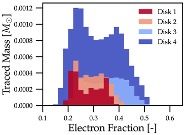
Translating this to the notation used for Parthenon histogram outputs means specifying for each histogram

• the field containing the Electron fraction as x_variable,

• the field containing the traced mass density as binned_variable, and

• enable weight_by_volume (to get the total traced mass).

Similarly, a 2D histogram (also referred to as phase plot) example may look like (from the yt Project documentation):

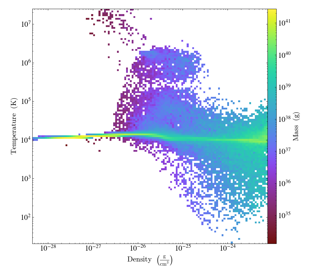
Translating this to the notation used for Parthenon histogram outputs means using

• the field containing the density as x_variable,

• the field containing the temperature as y_variable,

• the field containing the mass density as binned_variable, and

• enable weight_by_volume (to get the total mass).

The following is a minimal example to plot a 1D and 2D histogram from the output file:

with h5py.File("parthenon.out8.histograms.00040.hdf", "r") as infile:
  # 1D histogram
   x = infile["myname/x_edges"][:]
   y = infile["myname/data"][:]
   plt.plot(x, y)
   plt.show()

   # 2D histogram
   x = infile["other_name/x_edges"][:]
   y = infile["other_name/y_edges"][:]
   z = infile["other_name/data"][:].T   # note the transpose here (so that the data matches the axis for the pcolormesh)
   plt.pcolormesh(x,y,z,)
   plt.show()

Ascent (optional)

Parthenon supports in situ visualization and analysis via the external Ascent library. Support for Ascent is disabled by default and must be enabled via PARTHENON_ENABLE_ASCENT=ON during configure.

In the input file, include a <parthenon/output*> block and specify file_type = ascent. A dt parameter controls the frequency of outputs for simulations involving evolution. Note that in principle Ascent can control its own output cadence (including automated triggers). If you want to call Ascent on every cycle, set dt to a value smaller than the actual simulation dt. The mandatory actions_file parameter points to a separate file that defines Ascent actions in .yaml or .json format, see Ascent documentation for a complete list of options.

Parthenon currently only publishes cell-centered variables to Ascent. Moreover, the published name of the field always starts with the base name (to avoid name clashes between multiple fields that may have the same [component] labels). If component label(s) are provided, they will be added as a suffix, e.g,. basename_component-label for all variable types (even scalars). Otherwise, an integer index is added for vectors/tensors with more than one component, i.e., vectors/tensors with a single component and without component labels will not contain a suffix. The definition of component labels for variables is typically done by downstream codes so that the downstream documentation should be consulted for more specific information.

A <parthenon/output*> block might look like:

<parthenon/output9>
file_type = ascent
dt = 1.0
actions_file = my_actions.yaml

see also the advection example input file and actions file.

Note by default “field filtering” is enabled for Ascent in Parthenon, i.e., only fields that are used in Ascent actions are published. There may be cases, where Ascent cannot determine which fields it needs for an action and will fail. In this case, add an ascent_options.yaml file to the run directory containing:

field_filtering: false

to override at runtime. See Ascent documenation for more information.

Postprocessing and data analysis

Native Parthenon-based

A rudimentary postprocessing option is available to analyze data in restart files within the downstream/Parthenon framework, i.e., making use of native compute capabilities.

To trigger this kind of analysis, restart with -a /PATH/TO/RESTART/OUTPUT (instead of -r). This will launch the standard driver as if a simulation would be restarted, but never call the main time loop. Only the callbacks UserWorkBeforeLoop are executed. Afterwards, all output blocks that have the parameter analysis_output=true are going to be processed including UserWorkBeforeOutput callbacks.

Note, the standard modifications to the original input parameters via the command line or via an input file apply. A typical use case is, for example, to calculate histograms a posteriori, i.e., a new output block is specified in a file called sample_hist.in with all necessary details (particularly the analysis_output=true parameter within said block) and then the data can be processed via -a /PATH/TO/RESTART/OUTPUT -i sample_hist.in.

Python scripts

openPMD outputs

Outputs written following the openPMD standard can be processed by any tool implemting the standard. For Python based analysis the most straightforward way is via the openPMD-api or even more easily via the openPMD-viewer that builds on the API (both can be installed via pip).

HDF5 outputs

The scripts/python folder includes scripts that may be useful for visualizing or analyzing data in the .phdf files. The phdf.py file defines a class to read in and query data. The movie2d.py script shows an example of using this class, and also provides a convenient means of making movies of 2D simulations. The script can be invoked as

python3 /path/to/movie2d.py name_of_variable *.phdf

which will produce a png image per dump suitable for encoding into a movie.

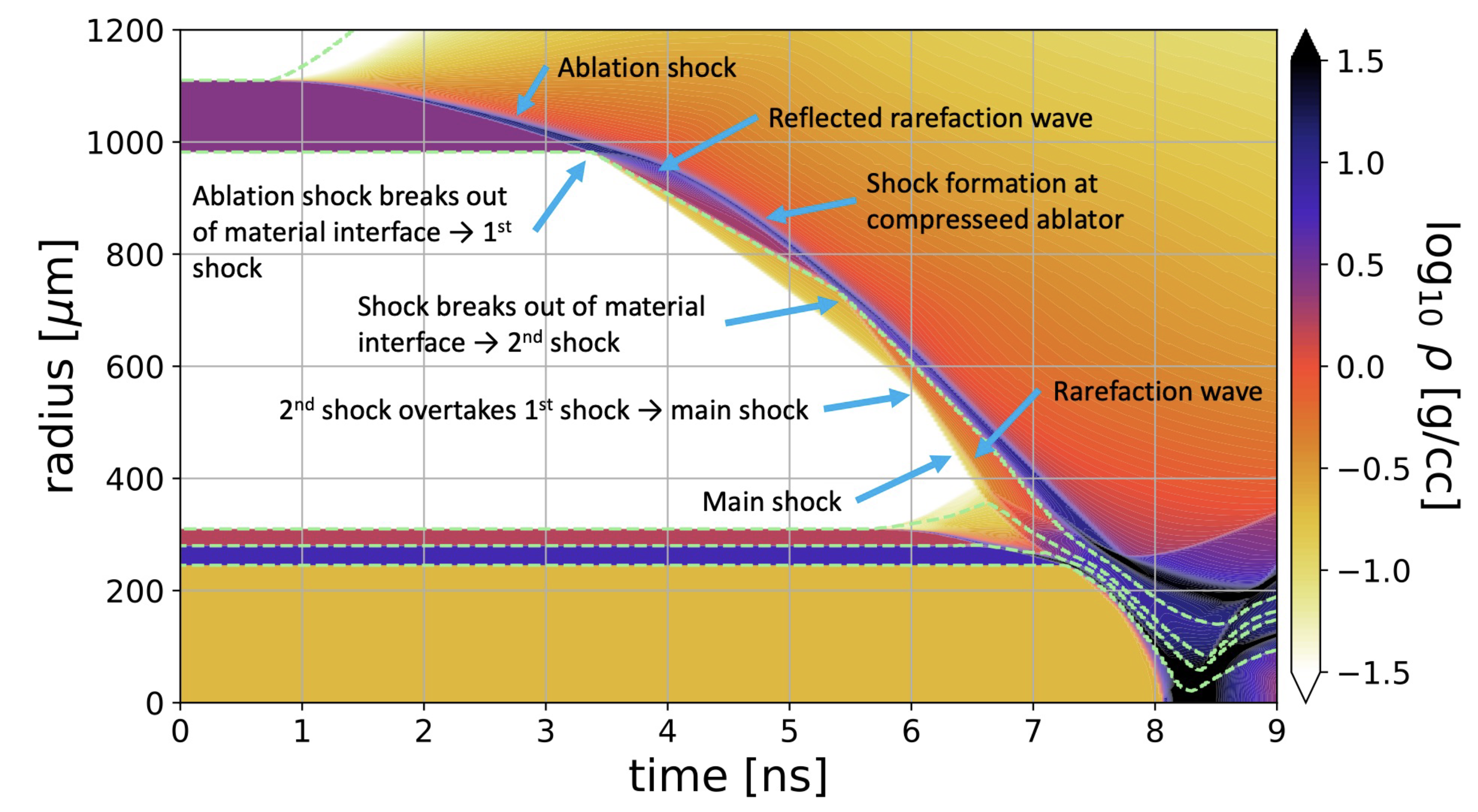
The contour1d.py script generates a spacetime plot of a field for 1D simulations. It may also be imported to provide tooling for building spacetime grids on a uniform covering mesh. It may be invoked as

python3 /path/to/contour1d.py name_of_variable *.phdf

This can be useful to plot 1D data as a function of time, especially for spherically symmetric problems. For example contour plots like this one, from a simulaiton of inertial confinement fusion, are possible with the script:

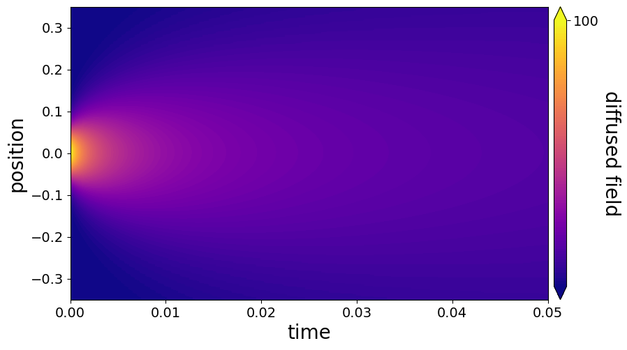
Here is an example run on our diffusion example in the parthenon examples folder:

Visualization software

Both ParaView and VisIt are capable of opening and visualizing Parthenon graphics dumps.

For HDF5 outputs, the .xdmf files should be opened. In ParaView, select the “XDMF Reader” when prompted.

For openPMD outputs, the native BP5 reader can be used to open the files. However, this may perform poorly (due to lack of automated mesh decomposition and load balancing). Thus, it is recommended to use the specific openpmd-visit-reader plugin for VisIt, which has robustly handled larger, multiple TB datasets.

Warning

Currently parthenon face- and edge- centered data is not supported for ParaView and VisIt. However, our python tooling does support all mesh locations.

Tying non-standard coordinates to visualization tools

By default, Parthenon outputs the positions of faces on each block in X1, X2 and X3 and assumes these correspond to the x, y, and z components of the nodes on the mesh. However, some applications may apply cooridnate transformations or use moving meshes. In these cases, the above strategy will not provide intuitive plots.

For these applications we provide a special Metadata flag. If you mark a node-centered 3-vector variable with the the flag Metadata::CoordinatesVec, and fill it with the x, y, and z values of your node positions, Parthenon will specify these values should be used by visualization software such as Visit or Paraview.

For example, in your package Initialize function, you might declare something like:

pkg->AddField("locations",
  Metadata({Metadata::Node, Metadata::CoordinatesVec, Metadata::Derived, Metadata::OneCopy},
  std::vector<int>{3}));

and then (trivially) if you set

pman.app_input->InitMeshBlockUserData = SetGeometryBlock;

for

void SetGeometryBlock(MeshBlock *pmb, ParameterInput *pin) {
  /* boiler plate to build a pack object */
  parthenon::par_for(DEFAULT_LOOP_PATTERN, "positions", DevExecSpace(), 0, pack.GetNBlocks() - 1,
  kb.s, kb.e, jb.s, jb.e, ib.s, ib.e,
  KOKKOS_LAMBDA(const int b, const int k, const int j, const int i) {
       const auto &coords = pack.GetCoordinates(b);
       pack(b, 0, k, j, i) = coords.X<X1DIR, parthenon::TopologicalElement::NN>(k, j, i);
       pack(b, 1, k, j, i) = coords.X<X2DIR, parthenon::TopologicalElement::NN>(k, j, i);
       pack(b, 2, k, j, i) = coords.X<X3DIR, parthenon::TopologicalElement::NN>(k, j, i);
  });
  return;
}

then the code will set the nodal values to their trivial coordinate values and these will be used for visualization. In a more non-trivial example, SetGeometryBlock might apply a coordinate transformation. Or actually evolve "locations".

Warning

Non-standard coordinates are not supported in XDMF for 1D meshes and Parthenon will revert to the traditional output in 1D.

Preparing outputs for yt

Support for openPMD outputs in yt is currently under development, see open PR so mileage may vary at the moment.

Parthenon HDF5 outputs can be read with the python visualization library yt as certain variables are named when adding fields via StateDescriptor::AddField and StateDescriptor::AddSparsePool. Variable names are added as a std::vector<std::string> in the variable metadata. These labels are optional and are only used for output to HDF5. 4D variables are named with a list of names for each row while 3D variables are named with a single name. For example, the following configurations are acceptable:

auto pkg = std::make_shared<StateDescriptor>("Hydro");

/* ... */
const int nhydro = 5;
std::vector<std::string> cons_labels(nhydro);
cons_labels[0]="Density";
cons_labels[1]="MomentumDensity1";
cons_labels[2]="MomentumDensity2";
cons_labels[3]="MomentumDensity3";
cons_labels[4]="TotalEnergyDensity";
Metadata m({Metadata::Cell, Metadata::Independent, Metadata::FillGhost},
           std::vector<int>({nhydro}), cons_labels);
pkg->AddField("cons", m);

const int ndensity = 1;
std::vector<std::string> density_labels(ndensity);
density_labels[0]="Density";
m = Metadata({Metadata::Cell, Metadata::Derived}, std::vector<int>({ndensity}), density_labels);
pkg->AddField("dens", m);

const int nvelocity = 3;
std::vector<std::string> velocity_labels(nvelocity);
velocity_labels[0]="Velocity1";
velocity_labels[1]="Velocity2";
velocity_labels[2]="Velocity3";
m = Metadata({Metadata::Cell, Metadata::Derived}, std::vector<int>({nvelocity}), velocity_labels);
pkg->AddField("vel", m);

const int npressure = 1;
std::vector<std::string> pressure_labels(npressure);
pressure_labels[0]="Pressure";
m = Metadata({Metadata::Cell, Metadata::Derived}, std::vector<int>({npressure}), pressure_labels);
pkg->AddField("pres", m);

The yt frontend needs either the hydrodynamic conserved variables or primitive compute derived quantities. The conserved variables must have the names "Density", "MomentumDensity1", "MomentumDensity2", "MomentumDensity3", "TotalEnergyDensity" while the primitive variables must have the names "Density", "Velocity1", "Velocity2", "Velocity3", "Pressure". Either of these sets of variables must be named and present in the output, with the primitive variables taking precedence over the conserved variables when computing derived quantities such as specific thermal energy. In the above example, including either "cons" or "dens", "vel", and "pres" in the HDF5 output would allow yt to read the data.

Additional parameters can also be packaged into the HDF5 file to help yt interpret the data, namely adiabatic index and code unit information. These are identified by passing true as an optional boolean argument when adding parameters via StateDescriptor::AddParam. For example,

pkg->AddParam<double>("CodeLength", 100,true);
pkg->AddParam<double>("CodeMass", 1000,true);
pkg->AddParam<double>("CodeTime", 1,true);
pkg->AddParam<double>("AdibaticIndex", 5./3.,true);

pkg->AddParam<int>("IntParam", 0,true);
pkg->AddParam<std::string>("EquationOfState", "Adiabatic",true);

adds the parameters CodeLength, CodeMass, CodeTime, AdiabaticIndex, IntParam, and EquationOfState to the HDF5 output. Currently, only int, float, and std::string parameters can be included with the HDF5.

Code units can be defined for yt by including the parameters CodeLength, CodeMass, and CodeTime, which specify the code units used by Parthenon in terms of centimeters, grams, and seconds by writing the parameters. In the above example, these parameters dictate yt to interpret code lengths in the data in units of 100 centimeters (or 1 meter per code unit), code masses in units of 1000 grams (or 1 kilogram per code units) and code times in units of seconds (or 1 second per code time). Alternatively, this unit information can also be supplied to the yt frontend when loading the data. If code units are not defined in the HDF5 file or at load time, yt will assume that the data is in CGS.

The adiabatic index can also be specified via the parameter AdiabaticIndex, defined at load time for yt, or left as its default 5./3..

For example, the following methods are valid to load data with yt

filename = "parthenon.out0.00000.phdf"

#Read units and adiabatic index from the HDF5 file or use defaults
ds = yt.load(filename)

#Specify units and adiabatic index explicitly
units_override = {"length_unit" : (100, "cm"),
                  "time_unit"   : (1,   "s"),
                  "mass_unit"   : (1000,"g")}

ds = yt.load(filename,units_override=units_override,gamma=5./3.)

The yt frontend for Parthenon is availble in yt >= 4.4.